Examples
This section lists some examples using cesiumpy and other packages. You
can find Jupyter Notebook of these exampless under GitHub repository
(maps are not rendered on GitHub. Download an run them on local).
Use with pandas
Following example shows retrieving “US National Parks” data from Wikipedia, then plot number of visitors on the map.
First, load data from Wikipedia using pd.read_html functionality. The data
contains latitude and longitude as text, thus some preprocessing is required.
>>> import pandas as pd
>>> url = "https://en.wikipedia.org/wiki/List_of_national_parks_of_the_United_States"
>>> df = pd.read_html(url, header=0)[0]

>>> locations = df['Location'].str.extract(u'(\D+) (\d+°\d+′[NS]) (\d+°\d+′[WE]).*')
>>> locations.columns = ['State', 'lat', 'lon']
>>> locations['lat'] = locations['lat'].str.replace(u'°', '.')
>>> locations['lon'] = locations['lon'].str.replace(u'°', '.')
>>> locations.loc[locations['lat'].str.endswith('S'), 'lat'] = '-' + locations['lat']
>>> locations.loc[locations['lon'].str.endswith('W'), 'lon'] = '-' + locations['lon']

>>> locations['lat'] = locations['lat'].str.slice_replace(start=-2)
>>> locations['lon'] = locations['lon'].str.slice_replace(start=-2)
>>> locations[['lat', 'lon']] = locations[['lat', 'lon']].astype(float)

>>> locations.head()
            State    lat     lon
0           Maine  44.21  -68.13
1  American Samoa -14.15 -170.41
2            Utah  38.41 -109.34
3    South Dakota  43.45 -102.30
4           Texas  29.15 -103.15

>>> df = pd.concat([df, locations], axis=1)
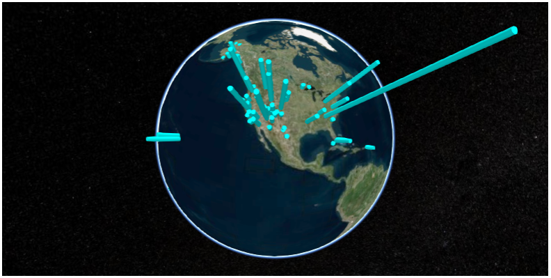
Once prepared the data, iterate over rows and plot its values. The below script adds
cesiumpy.Cylinder which height is corresponding to the number of visitors.
>>> import cesiumpy

>>> options = dict(animation=True, baseLayerPicker=False, fullscreenButton=False,
...                geocoder=False, homeButton=False, infoBox=False, sceneModePicker=True,
...                selectionIndicator=False, navigationHelpButton=False,
...                timeline=False, navigationInstructionsInitiallyVisible=False)

>>> v = cesiumpy.Viewer(**options)

>>> for i, row in df.iterrows():
...     l = row['Recreation Visitors (2014)[5]']
...     cyl = cesiumpy.Cylinder(position=[row['lon'], row['lat'], l / 2.], length=l,
...                             topRadius=10e4, bottomRadius=10e4, material='aqua', alpha=0.5)
...     v.entities.add(cyl)

>>> v
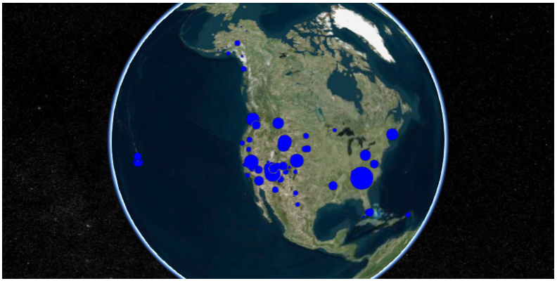
If you want bubble chart like output, use Point entities.
>>> v = cesiumpy.Viewer(**options)
>>> for i, row in df.iterrows():
...     l = row['Recreation Visitors (2014)[5]']
...      p= cesiumpy.Point(position=[row['lon'], row['lat'], 0],
...                        pixelSize=np.sqrt(l / 10000), color='blue')
>>> v.entities.add(p)
>>> v
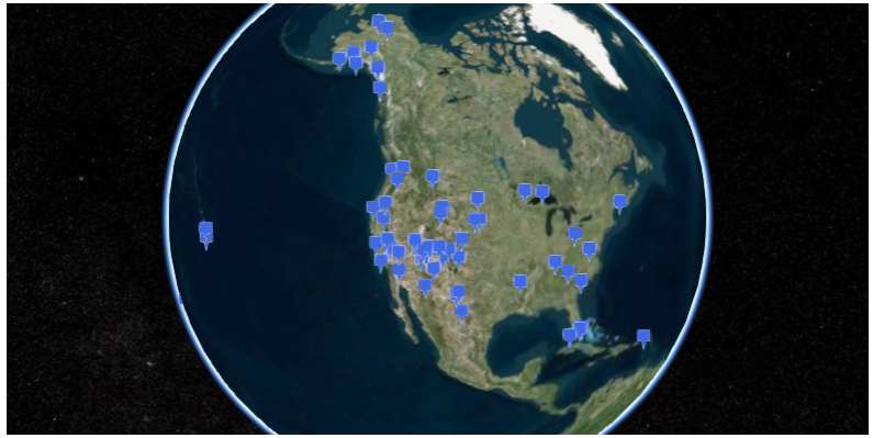
Using Billboard with Pin points the locations of National Parks.
>>> v = cesiumpy.Viewer(**options)
>>> pin = cesiumpy.Pin()
>>> for i, row in df.iterrows():
...     b = cesiumpy.Billboard(position=[row['lon'], row['lat'], 0], image = pin, scale=0.4)
>>> v.entities.add(b)
>>> v
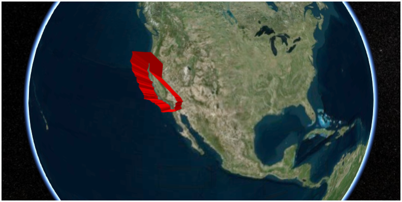
Use with shapely / geopandas
Following example shows how to handle geojson files using shapely, geopandas and cesiumpy.
First, read geojson file of US, California using geopandas function.
The content will be shapely instance.
>>> import geopandas as gpd

>>> df = gpd.read_file('ca.json')
>>> df.head()
  fips                                           geometry      id        name
0   06  POLYGON ((-123.233256 42.006186, -122.378853 4...  USA-CA  California

>>> g = df.loc[0, "geometry"]
>>> type(g)
shapely.geometry.polygon.Polygon
We can use this shapely instance to specify the shape of cesiumpy instances.
The below script adds cesiumpy.Wall which has the shape of California.
>>> import cesiumpy

>>> options = dict(animation=True, baseLayerPicker=False, fullscreenButton=False,
...                geocoder=False, homeButton=False, infoBox=False, sceneModePicker=True,
...                selectionIndicator=False, navigationHelpButton=False,
...                timeline=False, navigationInstructionsInitiallyVisible=False)

>>> v = cesiumpy.Viewer(**options)
>>> v.entities.add(cesiumpy.Wall(positions=g,
...                              maximumHeights=10e5, minimumHeights=0,
...                              material=cesiumpy.color.RED))
>>> v
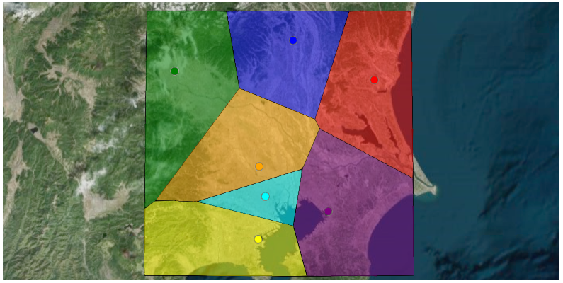
Use with scipy
cesiumpy has spatial submodule which offers functionality like scipy.spatial. These function
requires scipy and shapely installed.
Following example shows Voronoi diagram using cesiumpy. First, prepare a list contains the geolocations of Japanese Prefectual goverments.
>>> import cesiumpy

>>> options = dict(animation=True, baseLayerPicker=False, fullscreenButton=False,
...                geocoder=False, homeButton=False, infoBox=False, sceneModePicker=True,
...                selectionIndicator=False, navigationHelpButton=False,
...                timeline=False, navigationInstructionsInitiallyVisible=False)

>>> points = [[140.446793, 36.341813],
...           [139.883565, 36.565725],
...           [139.060156, 36.391208],
...           [139.648933, 35.857428],
...           [140.123308, 35.605058],
...           [139.691704, 35.689521],
...           [139.642514, 35.447753]]
Then, you can create cesiumpy.spatial.Voronoi instance passing points. Using get_polygons method returns the list of cesiumpy.Polygon instances. Each Polygon represents the region corresponding to the point.
>>> vor = cesiumpy.spatial.Voronoi(points)
>>> polygons = vor.get_polygons()
>>> polygons[0]
Polygon([140.70970652380953, 35.78698294268851, 140.06610971077615, 36.06956523268194, 140.03367654609778, 36.1229878712242, 140.27531919409412, 36.730815523809525, 140.70970652380953, 36.730815523809525, 140.70970652380953, 35.78698294268851])

>>> v = cesiumpy.Viewer(**options)
>>> colors = [cesiumpy.color.RED, cesiumpy.color.BLUE, cesiumpy.color.GREEN,
...           cesiumpy.color.ORANGE, cesiumpy.color.PURPLE, cesiumpy.color.AQUA,
...           cesiumpy.color.YELLOW]

>>> for p, pol, c in zip(points, polygons, colors):
...     b = cesiumpy.Point(position=(p[0], p[1], 0), color=c)
...     v.entities.add(b)
...     pol.material = c.set_alpha(0.5)
...     pol.outline = True
...     v.entities.add(pol)
>>> v.camera.flyTo((139.8, 36, 3e5))
>>> v
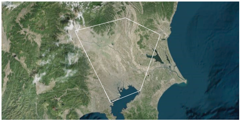
Next example shows to draw convex using cesiumpy. You can use cesiumpy.spatial.ConvexHull class, then use get_polyline method to get the cesiumpy.Polyline instances. Polyline contains the coordinates of convex.
>>> conv = cesiumpy.spatial.ConvexHull(points)
>>> polyline = conv.get_polyline()
>>> polyline
Polyline([139.060156, 36.391208, 139.642514, 35.447753, 140.123308, 35.605058, 140.446793, 36.341813, 139.883565, 36.565725, 139.060156, 36.391208])

>>> v = cesiumpy.Viewer(**options)
>>> v.entities.add(polyline)
>>> v.camera.flyTo((139.8, 36, 3e5))
>>> v